Predicting Global and Regional Petroleum Consumption Trends Part 3: The Former Soviet Union

This continues the series of PIE (Production, Imports and Exports) analysis to predict future petroleum consumption, this time, for The Former Soviet Union (FS).  For background, see Part 1 and for a more detailed walk-through of how the analysis is done, see Part 2. 

Figure 6 presents the reported production, consumption and net exports rates (dark blue, bright red and dark green open circles respectively) and the corresponding nonlinear least squares analysis (NLLS) best curves (solid lines with the same respective colors ). 

 Similar to the ME, reported production rate data for the FS shows two separate peaks in production, and I modeled this data with two separate logistic equation NLLS fits to the 1965-97 time span and to the 1998-2011 time span.  The consumption rate data in the FS are similarly bimodally distributed, and therefore, I also modeled these data with two separate logistic equation NLLS fits to the 1965-97 time span and to the 1998-2011 time span.

The best fit parameters of Q_o, Q_∞ and the rate constant, "a," from these logistic equation fits are summarized in Table 3 below:

Table 3 summary of best fit parameter for production and consumption for FS
	Qo (bbs)	Q∞ (bbs)	a (yr-1)
Production 1965-1997	14	151	0.12
Production 1998-2011	20	143	0.14
Consumption 1965-1997	9.0	102	0.12
Consumption 1998-2011	117	1007	0.012

Although NLLS best fit to the production data 1998-2011 time span is fairly similar to analysis to my earlier ELM analysis for the FS in Estimating the End of Global Petroleum Exports, the NLLS best fit to the consumption data is quite different.  The best fit to the consumption data for the 1998-2011 time span (red line), suggests a several times larger ultimately recoverable reserve (Q_∞) than in “Estimating the End.”  This is due to the continuing up-tick in FS’s consumption rates for the past two years.  The NLLS best fit looks more like a linear regression line but that is what the data trend is suggesting, and so, I am bound to go with this trend. 

A consequence of this higher rate of consumption is that “net exports” (again defined here as total production rate minus total consumption rate) hits zero in 2027; that’s a full six years earlier than what was predicted in “Estimating the End.” 

What does my PIE analysis do with the data for FS?  As you will see almost the opposite trends are obtained.

I am going to go through this much faster than I did for ME, especially the steps that are about the same as described in detail in Part 2.

Predicting Export Rates from FS to other Regions

Figure 7 shows the relationship between petroleum production rates and export rates for the FS, as already worked out in my previous study from last month ago.   This is actual the same as Figure 7 in Part 2 the “Relationship between Petroleum Exports and Production.”

Unlike ME, whose total export rates are trending downwards, FS’s total export rates relative to its total production rate are on a strong upward trend (black Xs and line, r²=0.80).  And, except for exports to SA and "UN" all of the other regions that receive exports (not ME, of course) are receiving ever-increasing proportions of FS production in the form of exports. 

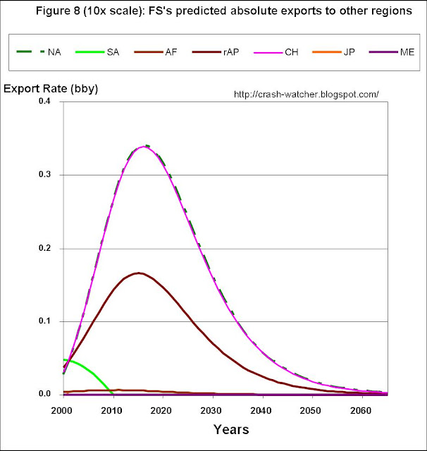
Figure 8 shows predicted regional asolute exports from FS to the other regions, based upon combining the production rate trends shown in Figure 6 with the export trend lines shown in Figure 7.

The most striking aspect to this plot is that it illustrate the huge proportions of the FS’s total exports (black line) that go to EU (blue line) as compared to any other region.  I suppose that one could look at this is two ways: EU is highly dependent on imports from the FS’s, or, FS is highly dependent on EU as an export destination.  Perhaps both are true.  As suggested by the trend lines in FIG. 7, FS's exports have been shifting towards NA, CH, JP and rAP, but these are much smaller amounts.  In fact to really see these trends, you have to expand the vertical scale 10 times:

In these figures I presented NA as a dashed line so that the export trends for NA and CH were both discernable.  It is interesting that these two regions are on virtually identical trend lines (oh, yes, I did indeed double check the results).  But these exports peak around 2016 and go down afterwards because by then FS’s production rates are in serious decline (FIG. 6, blue line).    Consequently FS never becomes a major petroleum supplier to the Asian regions (CH, rAP, JP) or NA.   

Some readers might wonder: what happen to EU as the FS’s exports go into decline? But I think one might equally winder: what happens to FS if it stays on its trend of ever-increasing exports as a fraction of total production?   

I will address this in a minute—but first there are some housing-keeping chores to take care of.  

Predicting Import Rates to FS from other Regions

Again, like ME, this is a non-issue—FS’s imports from individual other regions are so small that the BP review doesn’t report it.  

Predicting Consumption Rates for FS based on the PIE analysis

I am not going to repeat the whole issue about normalizing the predicted consumption and NET exports (which again like ME correspons to absolute exports, since FS has substantially no imports) based upon a comparison of reported consumption rate versus the consumption calculated from PIE for the time range (2000 to 2011) where I have actual data.  Briefly, for FS, the calculated consumption rate is 0.251 ± 0.123 bby higher than the reported consumption rate.  This is in contrast to ME where the calculated consumption rate was 0.403 ± 0.168 lower than the reported consumption rate.  Therefore my normalization for FS consisted of subtracting 0.251 bby from the calculated prodution rate, and, adjusting total net export rate upwards by this same amount—this in turn implies that the individual absolute exports to each of the other regions should be adjusted upwards proportionally so as to sum up to the adjusted total export rate amount.

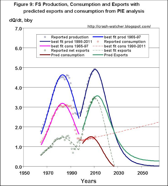
Alright then, Figure 9 again shows the production, consumption and net export data, and corresponding best fit curves, the later two curves now shown as dashed lines.  Added is the predicted export (light green solid line) and consumption (blood red solid line) prediction curves based on my PIE analysis. 

Figure 9 shows that, if FS’s production rate follows the logistic equation best fit (solid blue line), and the ever-increasing export rate trend continues along the lines shown in Figures 7 and 8, then the predicted total export rate curve (solid green line) is extended well past 2027 (dashed green line). 

The consequence of this however would be quite devastating for FS—now consumption drops to zero in 2027!  This is partly due to my normalization factor of -0.251 being applied to the consumption data—but even without normalization consumption goes to zero in 2038.  

This looks like the opposite of what the ELM analysis suggests in Figure 6. Now instead of unfettered increasing domestic consumption until hitting the production wall as suggested by the ELM analysis, the PIE analysis in Figure 9 suggests decreased consumption rates in order to sustain exports, until export hit the production rate wall.  The reason why the PIE analysis suggests this is due to the export trends revealed by the analysis supporting Figure 7. 

It is not realistic to think that FS would be able continue exporting at its present ever-increasing rate, even those that is what the trend line (black line, r²=0.8) in Figure 7 suggests. But at what point does would the present export trend end?  

I have some ideas about this, and, I will address this issue later on in the series, after completing the initial survey of all nine regions.  

For now, except for one adjustment, let’s just go with what the data trends are and see where this leads us. Consider this an upper boundary scenario, corresponding to the maximum that FS could possibly export, given its predicted production rate and current export trends.  

The one adjustment that I do want to make is analogous to the adjustment I made for ME.  In the context of Figures 4 in Part 2, I noted that ME’s consumption rates, predicted from the PIE analysis, actually exceeded production in about 2056.  This is unrealistic because ME substantiallydoesn’t import  any petroleum.  Therefore I adjusted ME’s petroleum consumption rate to match its production rate from 2056 and on.  

Here, for FS as illustrated in Figure 9, it is the export rate that exceeds the production rate in 2027.

Again this is unrealistic because FS substantially doesn’t import any petroleum.  Therefore I adjusted FS’s petroleum export rate to match its production rate from 2027 and on.  The result of this adjustment is presented in Figure 10.

Specifically, here’s how those exports to the other eight regions, previously presented in Figure 8, now look like, with the restriction that FS’s total export rate can’t exceed its production rate.  

As Compared to Figure 8, you can see that after 2027, exports to the other regions tail off more steeply, to match the rate of decline in the production rate.   

Of course, this doesn’t do anything to the prediction that FS’s consumption rates hit zero in 2027. 

But, having a more realist export rate prediction for FS is very important for subsequent PIE analysis for the other regions, because many of those other regions depend upon FS for imports.  

---------------------------------

Next time, in October, I will be back to present the PIE analysis of predicted consumption for Africa.